wEB aPPENdIX fOR rESEARCH DESIGN EXPLAINED Interpreting
ordinal and DisORDINAL INTERACTIONS
© 2006-2022, Mark Mitchell and Janina Jolley.
All Rights Reserved.
Interpreting Ordinal and Disordinal interactions
You do a 2 X 2 experiment and get an interaction. How do you make sense of that interaction?
The easiest way
to make sense of it is to graph your two simple main effects.[1]
Because you have a significant interaction, the lines representing these simple
main effects will have different slopes, reflecting the fact that the treatment
appears to have one effect in one condition, but a different effect in another
condition. In other words, because you have a significant interaction, the lines in
your graph will not be parallel.
Closer
inspection of these nonparallel lines will tell you whether you have an ordinal
interaction or a disordinal (crossover) interaction.
Ordinal Interactions May Mean That the Amount of Effect One Treatment Has Depends on the Level of the Other Treatment
Suppose that your nonparallel lines are sloping in the same
direction but do not actually cross. For example, both of the lines may slope
upward, but one of the lines has a steeper slope. Or, both of the lines may
slope downward, but one has a steeper slope. In either case, you have an ordinal interaction.
Ordinal interactions suggest that a treatment has a more intense effect in one condition than another. For example, you would find an ordinal interaction if a treatment was more effective for one type of patient than for another. You would also find an ordinal interaction if a teaching strategy helped both shy and outgoing children but helped outgoing children more. In the Figure below, you can see another example of an ordinal interaction: Exercise boosted participants’ calorie consumption by only 200 calories in the no-caffeine condition, but it boosted calorie consumption by 800 calories in the caffeine condition.
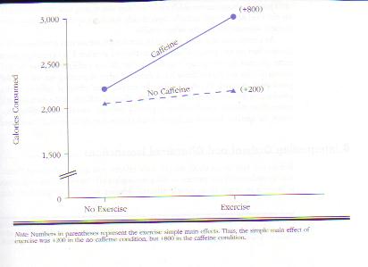
In this case,
the ordinal interaction seems to suggest that combining two independent
variables (caffeine and exercise) produces
larger than expected effects. The combination is greater than the sum of its
parts.
There are cases, however, where
ordinal interactions suggest that combining treatments is less effective than
you would expect from knowing the factors’ individual effects. That is, some
ordinal interactions result from the combination of treatments being less than
the sum of the effects of the individual treatments.
To sum up, some
ordinal interactions may reflect a treatment
having more of an effect when combined with another treatment whereas other ordinal
interactions may reflect a treatment having more of an effect when
another treatment is not around. All ordinal interactions suggest that a factor
appears to have more of an effect in
one condition than in another condition.
Ordinal Interactions May Be Measurement-Induced Mirages
We say appears to
have more of an effect because it is not easy to determine whether a variable
had more of a psychological effect in one condition than in another. For
example, to state that the psychological difference between 2,200 calories and 2,000 calories
is less than the difference between 3,000 calories and 2,200 calories, you must
have at least interval scale data: data in which the differences between
consecutive numbers always represent the same psychological difference. For
example, the difference between a score
of “1” and a score of “2” on the measure must be the same—in terms of the
characteristic that you are trying to measure— as the difference between 6 and
7. (To learn more about interval scale data, see Chapter 6.)
If you are
interested only in number of calories consumed, you can confidently say that
caffeine has more of an effect in the exercise condition than in the no-exercise
condition. It seems obvious that 800 calories (the difference in calorie
consumption between the exercise/caffeine group and the exercise/no-caffeine
group) is more than 200 calories (the difference in calorie consumption between
the no-exercise/caffeine group and the no-exercise/no-caffeine group).
However, if you are using calories consumed as a measure of how hungry people
felt, your measure may not be interval. Specifically, if you do not have a
one-to-one correspondence between number of calories consumed and degree of
perceived hunger, your data are not interval. Instead, your data are probably
ordinal: higher scores indicate more of a quality but equal differences between
scores do not necessarily indicate equal differences in the characteristic
allegedly being measured. For example, it may take the same increase in
perceived hunger to make a person who normally eats 2,000 calories consume an additional
200 calories as it does to get someone who would normally eat 2,200 calories to
eat an additional 800 calories. If it does, then the ordinal interaction
depicted in the previous graph is an artifact (an unintended result) of
calories consumed being an ordinal, rather than an interval, measure of hunger.
In that case, if you had used an interval scale measure of hunger, you would
not have obtained an interaction.
To visualize how
scale of measurement can affect our findings, consider the table below. The
first couple of rows of that table are quite similar to the results we just
discussed. For example, if you look at calories consumed, you see that there is
an ordinal interaction: The simple main effect of exercise in the no caffeine
condition (200) is less than the simple main effect of exercise in the caffeine
condition (800). This interaction may be due to exercising boosting feelings of
hunger more in the caffeine condition than in the no-caffeine condition. If this
is the case, if we repeated the study using a 1-9, interval rating scale measure
of hunger, we would again find an interaction. We have depicted that state of
events in the table's third row. However, what if calorie consumption doesn’t
map so nicely onto hunger? In that case, as you can see from the
table's last row, when we used an interval scale measure of hunger, we
might not obtain an interaction. Instead, we might find that the simple main effect of exercise would
be the same in both the no caffeine and caffeine conditions.
|
|
No
caffeine/ No
exercise |
No
caffeine/ Exercise |
Caffeine/ No
exercise |
|
|
Caffeine/ Exercise |
1st simple main effect |
2nd simple main effect |
|
Calories consumed |
2,000 |
2,200 |
2,400 |
2,600 |
2,800 |
3,000 |
2,200 –
2,000
= 200 |
3,000 –
2,400 = 600 |
|
Possible hunger scores on a 1-9 scale if
calories are an interval measure of hunger |
4 |
5 |
6 |
7 |
8 |
9 |
5 – 4 = 1 |
9 –
6
= 3 |
|
Possible hunger scores on a 1-9 scale if calories
are an ordinal measure of
hunger |
4 |
5 |
5.33 |
5.66 |
5.99 |
6.33 |
5 - 4 = 1 |
6.33 –
5.33 = 1 |
To see how you
might get an ordinal interaction even when the effect of combining two
variables produces nothing more than the sum of their individual effects, look
at figures “A” and “B” below. In Figure (A),
the lines are not parallel and thus indicate an interaction. But look
at the bottom Figure (B), which is a graph of the same data. In Figure B, the
lines are parallel, indicating no interaction.
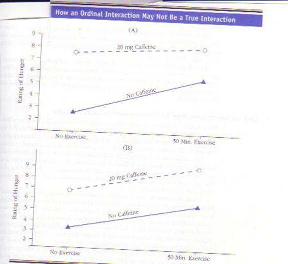
The first graph
depicts an interaction because it, like most graphs you have seen, makes the
physical distance between 3 and 4 equal to the distance between 7 and 8. However, by
doing this, the author of the graph assumes that the psychological distance
between 3 and 4 is the same as the psychological distance between a score of a 7
and a score of an 8. That is, the assumption is that the data are
interval. If the assumption that the data are interval is correct, then caffeine
makes participants feel hungrier in the exercise condition than it does in the
no-exercise condition.
The second graph (B) shows what can happen if we, rather than buying the assumption that these data are interval, suppose that we have ordinal data. Specifically, the graph shows what happens when the difference between a “7” and an “8” rating is greater—in terms of how much hunger people feel—than the difference between a “3” and a “4” rating. In that case, at the psychological level, caffeine’s effect on the subjective state of “feeling hungry” is the same in the exercise condition as it is in the no-exercise condition. Thus, even though there is an interaction at the statistical level, there is not an interaction at the psychological level: Although caffeine has more of an effect the number of physical calories consumed in the exercise condition, caffeine has the same psychological effect in both conditions. In other words, seeing that the treatment makes a greater change in participants’ scores in one condition doesn’t necessarily mean that the treatment makes a greater change in participants’ feelings: The numbers can hide a psychological truth.
When to Suspect That an Ordinal Interaction Is an Artifact of Having Ordinal Data
As you have seen, ordinal interactions may be nothing more
than an illusion caused by having ordinal, rather than interval, data. Because
you can rarely be sure that you have interval data, you should always be
cautious when interpreting ordinal interactions. However, you should be
especially cautious if you have reason to believe that your data are ordinal.
When Data are Ranks or Scores on Some Other Ordinal Measure
If your data come from having participants rank items from lowest
to highest, you have ordinal data. You can’t say that the difference between
something ranked “1” and something ranked “2” is the same as the difference
between something ranked “3” and something ranked “4” (see Chapter 6).
When Scores Suggest that Either
Ceiling or Floor Effects Are Likely
Because ordinal data make ordinal interactions difficult to
interpret, you may want to avoid using ordinal measures. Unfortunately,
however, avoiding ordinal data is not as easy as avoiding ordinal measures.
Even a measure that seems like it should provide interval data may end up
providing ordinal data.
To understand
how an interval scale measure could produce ordinal data, imagine a typical
bathroom scale. Normally, it would provide interval data. However, what if you
were measuring football players on it? Your scale would provide interval
measurement to those players who weighed less than 250 pounds (or whatever your
scale went up to). However, everyone 250 and above would, according to your
scale, weigh 250. Thus, you would know that someone who, according to your
scale, weighed 250 was heavier than someone weighing 245, but you wouldn’t know
how much heavier.
Not only would
your scale fail you at extremely high weights, it would also fail you at
extremely low weights. Thus, if you were weighing the food on football players’
plates, your scale would not provide accurate weights.
In technical
terminology, your bathroom scale has two weaknesses. First, its ceiling (the highest score participants
can receive) of 250 pounds is too low to accurately weigh some of the heavier football
players. Second, its floor (the
lowest score participants can receive) of five pounds is too high to accurately
measure objects less than 5 pounds.
The scale’s low
ceiling could hide the effect of a treatment. For example, suppose the heavy
football players are put on a weightlifting program that makes them even
heavier. Although the treatment works, the results would not show up on the
bathroom scale: The heavy players would, according to that scale, still “weigh”
250 pounds. In technical jargon, your results are misleading because of a ceiling effect: the effect of a
treatment or combination of treatments is underestimated because the dependent
measure is not sensitive to values above a certain level.
Just as the scale's low
ceiling could hide a treatment's effect, so too could the scale’s high
floor. For example, suppose the
football players are rewarded for putting less food on their plates, and the
reward system works. However, the researcher measures the amount of food on the
plate by using a bathroom scale that can’t accurately weigh anything under 5
pounds. The measure’s high floor makes it look like the players aren’t eating
less. In technical jargon, our results are misleading because of a floor effect: The effects of the
treatment or combination of treatments is underestimated because the dependent
measure places too high a floor on what the lowest response can be.
As you have seen, ceiling and
floor effects can make it seem like an effective treatment has no effect. In
addition, ceiling and floor effects can make it seem like an effective
treatment has a strong effect for one group but no effect for another group.
Let’s see how a
ceiling effect could make it look like a treatment that is equally effective
for two groups is only effective for one of the groups. Let’s start by
supposing that both light and heavy football players are put on a weightlifting
program. Furthermore, suppose that both groups gain 20 pounds. The light
football players go from 180 to 200 pounds; the heavy players go from 300 to
320. According to the bathroom scale, the light players gain 20 pounds
(180–200), but the heavy football players haven’t gained a pound. The scale
still has them all weighing 250 pounds. In this case, a ceiling effect made it
look like weightlifting has more of an effect on light than on heavy players,
even though weightlifting’s effect is the same for both types of players. That
is, due to a ceiling effect, our scale gave us an ordinal interaction when we
should not have had any interaction.
Like bathroom
scales, psychological scales may be plagued by low ceilings and high floors.
Thus, as with extreme scores on our bathroom scale, extreme scores on a
psychological measure may be misleading. Some of the low scorers may deserve
much lower scores, but the measure is unable to give it to them. In a sense,
the “floor” (the lowest score they can receive) is too high. Or, some of the
high scorers might, if given a chance, score much higher than the others—but the
measure doesn’t give them that chance. In such a case, the “ceiling” (the
highest score they can receive) is too low.
Thus far, you
know that ceiling and floor effects can contaminate your results. If your
measure’s ceiling is too low, ceiling effects may be contaminating your
results. If your measure’s floor is too high, floor effects may be
contaminating your results. In the next sections, you will learn (a) when to
suspect that a ceiling or floor effect is affecting your results and (b) how
ceiling and floor effects contaminate your results. Thus, after reading the
next section, you will be appropriately cautious when interpreting ordinal
interactions.
When to Suspect That an Ordinal Interaction Is Due to Ceiling Effects.
If a group’s average scores are quite high, you should
suspect that your ordinal interaction may be due to ceiling effects. Ceiling
effects occur when the measure does not allow participants to score as high as
they should For example, in the picture
below, the gym’s ceiling is only 10 feet high, so coaching can’t make Larry
jump any higher than 10 feet.
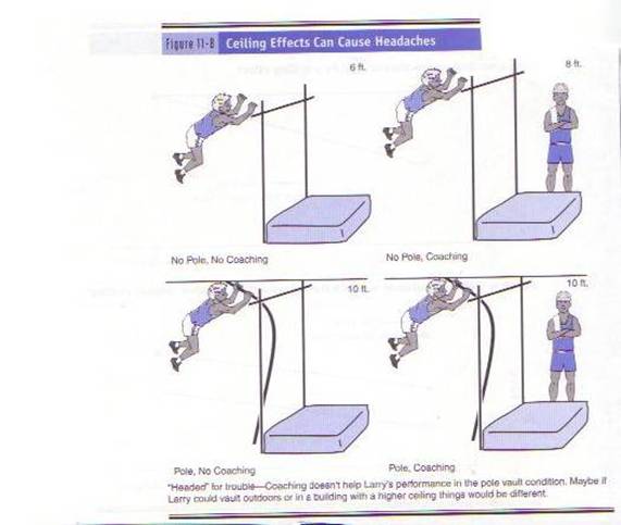
To take a more realistic example, imagine an extremely easy
knowledge test, in which half the class scores 100%. The problem with such a
test is that we can’t differentiate between the students who knew the material
fairly well and the students who knew the material extremely well. The test’s
“low ceiling” did not allow very knowledgeable students to show that they knew
more than the somewhat knowledgeable students.
To see how a
ceiling effect can create an ordinal interaction, consider the following
experiment. An investigator wants to know how information about a specific
person affects the impressions people form of that person. The investigator
uses a 2 (information about a stimulus person’s traits [no information versus
extremely positive information]) X 2 (information about a stimulus person’s
behavior [no information versus extremely positive information]) factorial
experiment. For the dependent measure, participants rate the stimulus person’s
character on a three-point scale (1 = below average, 2 = average, 3 = above
average).
As you can see
from the top of the next figure (Figure a), the investigator obtains an ordinal
interaction. The interaction suggests that getting information about a specific
person’s behavior has less of an impact if participants already have
information about that person’s traits. In fact, the interaction suggests that
if participants already know about the stimulus person’s traits, information
about the person’s behavior is worthless.
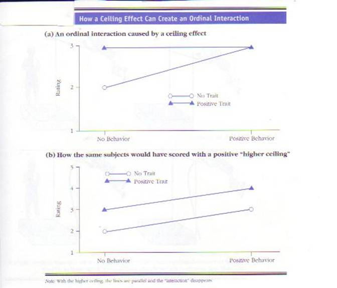
The problem in
interpreting this interaction is that the results could be due to a ceiling
effect. For example, participants may feel that a
person with a favorable trait is a 3 (above average) and a person with both a
favorable trait and a favorable behavior is a 4 (well above average), but the highest rating they can give a person is a 3.
In short, the highest rating (above average) on this scale—the ceiling response—is not
high enough.
By not allowing
participants to rate the stimulus person as high as they wanted to, the
investigator did not allow participants to rate the positive trait/positive
behavior person higher than either the positive trait/no behavior person or the
positive behavior/no trait person. Thus, the investigator’s ordinal interaction
was due to a ceiling effect. In other words, the interaction is due to the
dependent measure placing an artificially low ceiling on how high a response
can be. As you can see from Figure b above, “raising the
ceiling” would eliminate this ordinal interaction.
When to Suspect that an Ordinal Interaction Is Due to Floor Effects.
Just as ceiling effects can account for ordinal
interactions, so can their opposites—floor effects. For example, suppose the
investigator uses the same three-point rating scale as before (1 = below
average, 2 = average, 3 = above average). However, instead of using no
information and extremely positive information, the investigator uses no
information and extremely negative information. The investigator might again obtain
an ordinal interaction (see the next figure). Again, the interaction would
indicate that adding behavioral information to trait information has little
effect on participants’ impressions. This time, however, the interaction could
be due to the fact that participants could not rate the stimulus person lower
than a “1” (below average). The problem is that the bottom rating—the
“floor”—is too high.
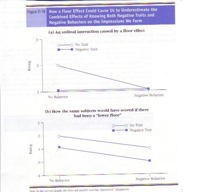
By not allowing
participants to rate the person as low as they wanted to, the investigator did
not allow participants to rate the negative trait/negative behavior stimulus
person lower than the negative trait/no behavior person or the negative
behavior/no trait person. Thus, the investigator’s ordinal interaction was due
to a floor effect. As you can see from the bottom half of the previous figure,
“lowering the floor” can eliminate some ordinal interactions.
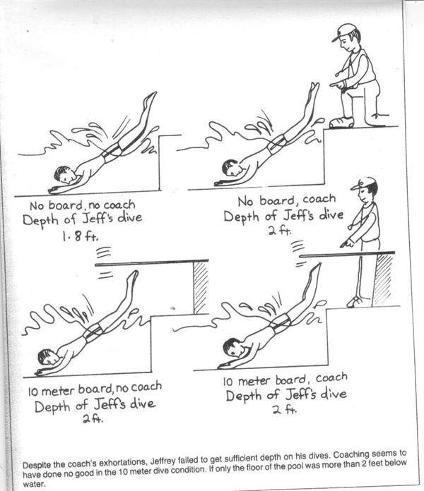
In short, as floor and
ceiling effects show, an ordinal interaction may reflect a measurement problem
rather than a true interaction. So, be careful when
interpreting ordinal interactions.
Disordinal (Crossover) Interactions Mean That The Type of Effect One Treatment Has Depends on the Level of the Other Treatment
You do not have to be so careful if
you have a crossover interaction. When you have a crossover interaction, as the
term “crossover interaction” suggests, the lines in your graph actually cross.
Crossover
interactions often indicate that a factor has one kind of effect in one
condition and the opposite kind of effect in another condition. For example,
you would have a crossover interaction if a therapy that helps patients who
have one kind of problem actually hurts patients who have a different kind of
problem. In the next figure, you can see another example of a cross-over
interaction: In the no-caffeine condition, exercise increases calorie consumption, but, in
the caffeine condition, exercise decreases
calorie consumption.
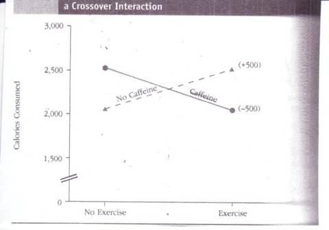
Crossover interactions are also called disordinal interactions because, unlike
ordinal interactions, they can’t be an artifact of having ordinal, rather than
interval, data. To understand why disordinal interactions can’t be due to
having ordinal data, let’s imagine a factorial experiment designed to determine
the effect of watching exercise videos and monitoring what one eats on physical
fitness. Specifically, middle-aged adult volunteers are assigned to one of four
conditions: (1) no video/no diet monitoring, (2) no video/diet monitoring, (3)
video/no diet monitoring, and (4) video/diet monitoring. After 6 weeks, fitness
is assessed.
The experimenter
assesses fitness by having the adults start one block east of
Unfortunately,
the experimenter did not check to make sure that all the blocks are equal in
length. Indeed, as it turns out, the blocks vary considerably in length.
Because some
blocks are very short and others are fairly long, the measure provides only
ordinal data. For example, we would know that someone who ran eight blocks ran
farther than someone who ran six blocks, but we wouldn’t know how much farther.
We would know one ran two blocks farther, but two blocks might be 100 feet or
it might be 10,000 feet. Therefore, if Mary runs eight blocks to Mabel’s six,
and Sam runs four blocks to Steve’s two, we cannot say that Mary outran Mabel
by the same distance as Sam outran Steve. Mary may have run 100 feet more than
Mabel, but Sam may have run 10,000 feet more than Steve.
How will the use
of an ordinal measure hurt the experimenter’s ability to interpret the results?
The answer to this question depends on the pattern of the results.
If the
researcher gets the ordinal interaction depicted in the next figure, there is a
problem because the apparent interaction may really be just an artifact of
having ordinal data. For example, the interaction could be due to the distance
between Seventh and Eighth Streets being longer than the distance between Third
and Fifth Streets. Thus, if the researcher had used an interval measure (such as
the number
of meters run), the researcher might not have found an interaction.
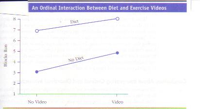
If, on the other
hand, the researcher gets the disordinal interaction depicted in the next figure, this interaction can’t be due to
having ordinal data. Even if the blocks are all of different lengths (i.e., the
measure is not interval), the interaction would still demonstrate that weight-monitoring
was more effective for the people watching the exercise videos than for those
not watching the videos.
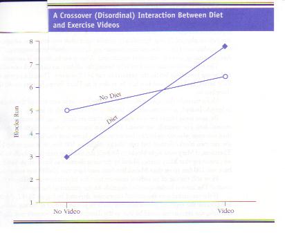
Regardless of the length of the blocks, we know that the
distance between
|
|
1st Street |
2nd Street |
3rd Street |
4th Street |
5th Street |
6th Street |
7th |
8th Street |
|
|
|
|
|
|
|
|
|
|
|
|
|
|
|
|
|
|
|
|
Conclusions About Interpreting Ordinal and Disordinal Interactions
To reiterate, disordinal interactions are less difficult to
interpret than ordinal interactions. Ordinal interactions are difficult to
interpret because there are always two possible explanations for an ordinal
interaction.
One possible
explanation is that the ordinal interaction really represents the fact that
combining your two independent variables produces an effect that is different
from the sum of their individual effects. Specifically, combining the factors
really has either less of, or more of, an effect than the sum of their
individual effects.
The second
possibility is that the apparent interaction is merely an artifact of ordinal
scale measurement (see Chapter 6 for a review of scales of measurement). If you
had more accurately measured the construct, you would not have found an
interaction. Therefore, if you want to say that an ordinal interaction
represents a true interaction, you need to establish that you have interval or
ratio data.
To illustrate
the difficulty of interpreting an ordinal interaction, suppose you find that a
treatment boosted scores from 15 to 19 in one condition, but from 5 to 8 in the
other. At the level of scores, you have an interaction: The treatment increased
scores more in one condition than in the other. But what about at the level of
psychological reality? Can you say that going from a 15 to a 19 represents more
psychological change than going from a 5 to an 8? Only if you have interval or
ratio scale data. In other words, with an ordinal interaction, you can only
conclude that the variables really interact if you can say that a one-point
change in scores at one end of your scale is the same thing (psychologically)
as a one-point change at any other part of your scale.
With crossover
(disordinal) interactions, on the other hand, you are not comparing differences
between scores on one part of your scale with differences between scores on an
entirely different part of your scale. Instead, you are making comparisons
between scores that overlap. For example, with a crossover interaction, you
might only have to conclude that the psychological difference between 10 and 30
is bigger than a difference between 15 and 19. Because the difference between
10 and 30 includes 15–19, you can conclude that the difference between 10 and
30 is bigger—even if you only have ordinal data. Thus, when you have a
crossover (disordinal) interaction, you can conclude that your variables really
do interact.